RCP CL Discrete Second Order Low Pass Filter Example

navigation bar

Table of Contents >Quanser Rapid Control Prototyping Toolkit >Examples >Basic Features >

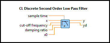
This example demonstrates how to use the RCP CL Discrete Second Order Low Pass Filter VI. For a detailed description of this VI and how it operates, please refer to the RCP CL Discrete Second Order Low Pass Filter help page.

System Requirements

Please refer to the Rapid Control Prototyping (RCP) Toolkit System Requirements to run this example. This example does not require any other hardware.

Configuring the Example

There is no configuration required to run this VI on a Windows PC. Once the RCP Discrete CL Second Order Low Pass Filter Example.lvproj is open, click the RCP Discrete CL Second Order Low Pass Filter Example.vi under My Computer and you are ready to execute the example.

Running the Example

Click on the VI Run button or select Run from the Operator menu to start the VI.

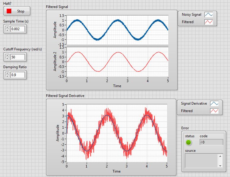
The top plot in the Filtered Signal chart displays the signal with the added noise and the bottom plot shows the filtered signal.

The blue trace in the Filtered Signal Derivative chart displays the theoretical/ideal derivative signal (without noise) while the red trace shows the filtered derivative of the original noisy signal.

Change the Cutoff Frequency and Damping Ratio parameters of the second-order filter and observe their effect on the filtered response. The Sample Time can be used to set the sampling interval (i.e. solver step size) of the VI.

Click on the Front Panel Stop button to stop the VI.

navigation bar